Statistics Fundamentals for Business Professionals 2026

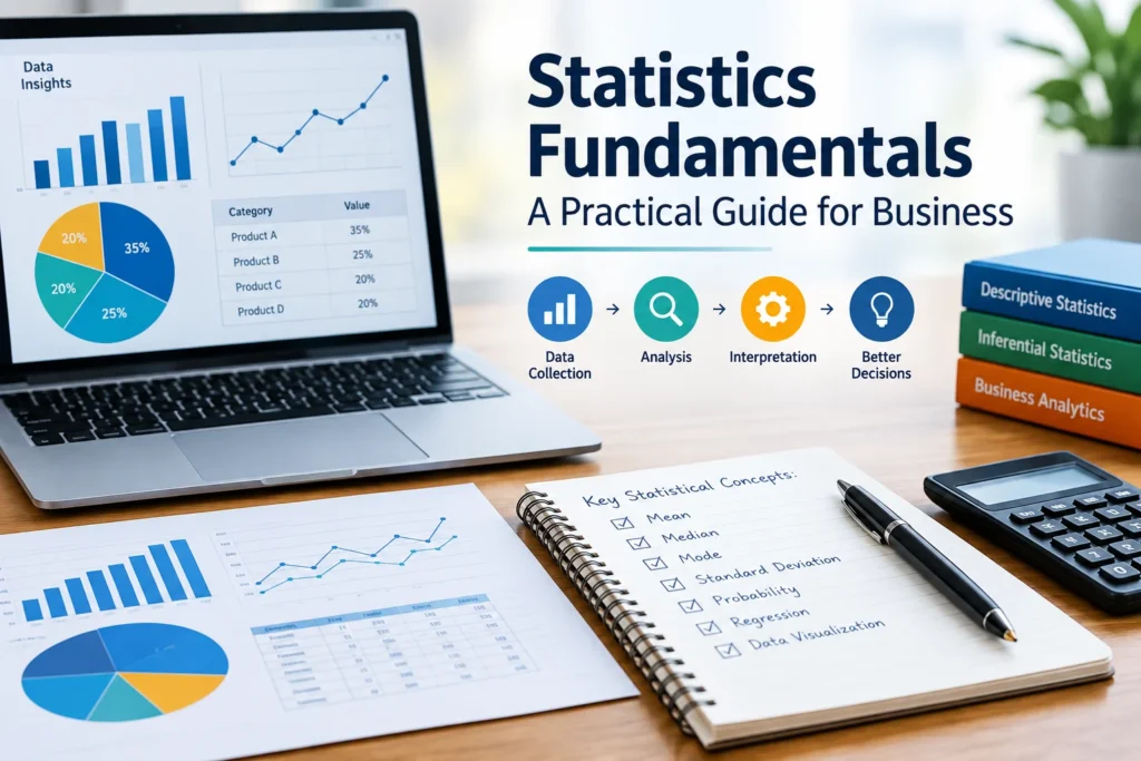
This guide covers the core ideas behind data-driven decisions: what the field is, how summaries differ from predictions, how to read averages and spread, why sampling matters, and what a p-value does and doesn’t tell you. No calculus required. Every concept comes with a workplace example, and you’ll finish with a short list of mistakes to dodge.

What Are Statistics Fundamentals?

Statistics fundamentals are the core methods for collecting, summarizing, and interpreting data so you can make decisions under uncertainty. Put simply, statistics turns a pile of numbers into a defensible answer.

The field splits into two halves. Descriptive statistics summarize what you already have. Inferential statistics use a smaller set of observations to draw conclusions about a larger group. Nearly everything else, from regression to A/B testing, builds on that split.

Why should a manager care? Because every dashboard is a statistical claim. Someone chose the average, the time window, and the sample. Knowing how those choices shape a number is the difference between reading a report and being led by it.

Descriptive vs. Inferential Statistics

Say you run a 40-person sales team. Last quarter’s average deal size was $18,500. That’s descriptive: it summarizes data you fully possess.

Now say you survey 200 of your 12,000 customers and find that 71% would renew. Claiming “about 71% of all customers would renew” is inferential. You’re jumping from a sample to a population, and that jump always carries uncertainty.

	Descriptive	Inferential
Question answered	What happened?	What’s likely true beyond this data?
Data used	The full dataset you hold	A sample from a larger group
Typical tools	Mean, median, charts	Confidence intervals, hypothesis tests
Main risk	Misleading summaries	Wrong generalizations

Know Your Data Types First

Before you calculate anything, ask what kind of data you’re holding. Categorical data sorts things into groups: product line, region, and satisfaction rating. Some categories have no order (region), and some do (a 1 to 5 rating scale). Numerical data counts or measures: units sold, hours logged, and revenue.

This matters because the type decides which method fits. Averaging ZIP codes produces a number with no meaning. Averaging revenue does. Most analysis errors I’d call “silent,” meaning the software still returns an answer, so nothing warns you that the question was wrong.

Averages and Spread: The Numbers Behind the Numbers

Three averages, three different stories. The mean adds everything up and divides by the count. The median is the middle value once you sort the list. The mode is the value that appears most often.

Here’s why the choice matters. Five deals close at $8,000, $9,000, $10,000, $11,000, and $62,000. The mean is $20,000, which sounds healthy. The median is $10,000, which is what a typical deal looks like. One whale dragged the mean upward. When data has outliers, as salaries, home prices, and deal sizes usually do, the median tells the truer story.

Averages hide variation, though. Two stores can both average $5,000 in daily sales. If one lands between $4,800 and $5,200 every day and the other swings between $1,000 and $9,000, you’d staff and stock them very differently. Spread measures that gap.

Standard deviation is the workhorse here. It roughly describes how far values typically sit from the mean, in the same units as your data. Variance is the same idea before taking the square root, so it’s harder to interpret. Range, the distance between your highest and lowest values, is quick but easily distorted by one extreme.

Never report a mean without some sense of spread. A lone number is half a sentence.

Sampling and Distributions: Why 1,000 Beats a Guess

You rarely get to measure everyone, so you sample. A good sample is random enough that every member of the group had a fair chance of inclusion. A bad one, like surveying only people who answered your email, bakes bias in before the first calculation.

Size matters too, with diminishing returns. For a yes/no survey question, a random sample of 1,000 gives a margin of error near three percentage points at 95% confidence. Drop to 100 people, and it balloons to roughly ten points. Doubling to 2,000 only trims it to about two. That’s why pollsters often stop near 1,000.

Then there’s the shape of the data. Many measurements pile up into a bell curve, the normal distribution. In it, about 68% of values fall within one standard deviation of the mean, 95% within two, and 99.7% within three. That’s the empirical rule, and it’s handy for spotting oddities. A value three standard deviations out deserves a second look.

The Central Limit Theorem explains why this shape appears so often. Average enough random samples, and those averages form a roughly normal pattern, even when the underlying data doesn’t. Around 30 observations is the usual rule of thumb, though heavily skewed data needs more. This one idea is what lets us build confidence intervals and run tests on messy real-world numbers.

Hypothesis Testing Without the Jargon

Back to that conversion rate. Version A converts at 4.0%, and version B at 4.4%. Was B truly better?

A hypothesis test starts by assuming nothing changed. That assumption is the null hypothesis. The alternative is that B really does differ. You pick a significance level in advance, commonly 0.05, collect the data, and calculate a p-value.

Here’s the part almost everyone gets wrong. A p-value of 0.03 doesn’t mean there’s a 3% chance the null is true. It means that if there were truly no difference, you’d see a gap this large or larger about 3% of the time. It measures surprise, not truth. And a small p-value says nothing about whether the difference is big enough to matter. A tiny lift can be “significant” with enough traffic and still not repay the engineering effort.

That’s why you should pair p-values with a confidence interval. A 95% interval gives a plausible range for the true effect. If your lift is 0.4 points with an interval of 0.1 to 0.7, it’s probably positive but could be small. Strictly speaking, the 95% describes the method: repeat the study many times, and about 95% of such intervals would capture the true value.

Want a deeper reference? The NIST/SEMATECH e-Handbook of Statistical Methods is a free, web-based book meant to help scientists and engineers apply statistical methods and better grasp the assumptions behind them. It’s dense, but it’s worth bookmarking. [YOUR EXPERIENCE: Add one or two sentences about a real test result or reporting decision you’ve handled.]

Correlation, Regression, and Causation

Two things moving together isn’t proof that one causes the other. Ice cream sales and sunburns both rise in July because heat drives both. Correlation, measured by a coefficient between -1 and +1, describes how tightly two variables travel together. Causation needs more, usually a controlled experiment where you change one thing on purpose and compare it against a group that didn’t get the change.

Regression goes a step further. Simple linear regression fits a line through your data so you can estimate an outcome from a predictor, such as revenue from ad spend. R-squared reports what share of the outcome’s variation the model explains. A high value isn’t automatically good, and a low one isn’t automatically bad. What counts as acceptable depends on the field, and predicting human behavior rarely gets near 1.

Five Mistakes That Skew Business Decisions

Reporting averages alone. Add the median and a spread measure.
Peeking at tests early. Check an A/B test daily and stop when it looks good, and you’ll inflate false positives. Set the sample size first.
Testing many things and reporting the winner. Test 20 unrelated metrics at 0.05, and there’s about a 64% chance at least one looks significant by luck alone.
Ignoring sample bias. A survey of your most engaged users describes engaged users.
Confusing significance with importance. Ask how big the effect is and what it’s worth.