What Is a VC Dimension? Vapnik-Chervonenkis Theory Explained

Why can a model fit its training data perfectly and still fail on new data? Vapnik-Chervonenkis theory, developed in the Soviet Union in the late 1960s and early 1970s, gave the first rigorous answer. Fit alone isn’t the issue. What matters is how much freedom a model has to fit anything at all. This guide covers the core ideas for undergrads: shattering, VC dimension, the generalization bound, and where it all shows up in practice.

What Is Vapnik-Chervonenkis Theory?

Vapnik-Chervonenkis (VC) theory is a branch of statistical learning theory that measures the capacity of a hypothesis class, meaning the set of functions an algorithm is allowed to choose from. Vladimir Vapnik and Alexey Chervonenkis laid out the central results in their 1971 paper on the uniform convergence of relative frequencies of events to their probabilities, published in Theory of Probability and Its Applications.

The question they tackled is easy to state. You train on a sample, so you only ever see training error. What you care about is errors in data you haven’t seen. How far apart can the two be? The answer is a bound that depends on the sample size and one number describing the class: its VC dimension.

Shattering: The Idea Behind VC Dimension

A set of points is shattered by a hypothesis class if the class can produce every possible labeling of those points. With n points and binary labels, that’s 2^n labelings.

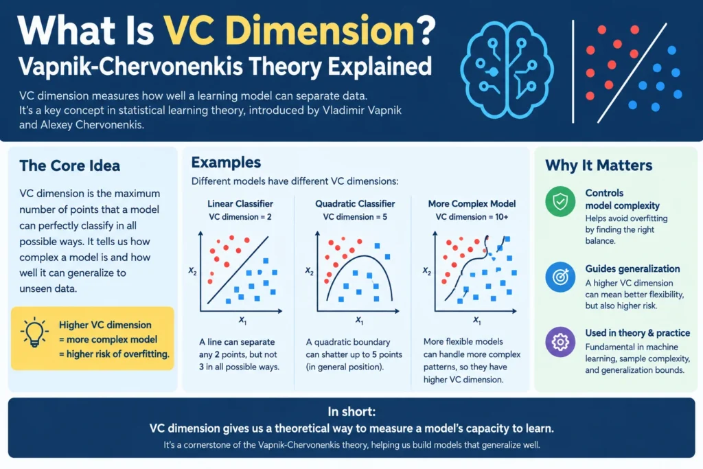
The VC dimension is the size of the largest set the class can shatter. If it shatters some set of d points but no set of d+1 points, the VC dimension is d. If it shatters arbitrarily large sets, the VC dimension is infinite.

Think of it as a capacity score. A high score means the class can bend to fit almost any pattern, noise included. A low score means it’s more constrained.

VC Dimension Examples You Can Check by Hand

Grab paper and test these.

• Thresholds on a line (label +1 if x ≥ t): VC dimension 1. Two points fail because you can’t label the left one + and the right one -.
• Intervals on a line: VC dimension 2. Three points fail on the pattern + – +.
• Lines in the plane: VC dimension 3. Three non-collinear points can be labeled all eight ways. Four points can’t, and the XOR arrangement is the classic failure.
• Linear classifiers in d dimensions: VC dimension d+1.
• Axis-aligned rectangles in the plane: VC dimension 4.

Notice the proof pattern. To show the VC dimension is at least d, you find one set of d points that gets shattered. To show it’s at most d, you prove that no set of d+1 points can be. Students mix those up all the time.

The Vapnik-Chervonenkis Generalization Bound

Here’s the payoff. For a class with VC dimension d and n training examples, with probability at least 1 − δ, the true error is at most the training error plus a complexity term that scales like the square root of (d·ln(n/d) + ln(1/δ)) / n. Exact constants differ between textbooks, so check your course’s version.

Read it slowly. The gap shrinks as n grows and widens as d grows. Finite VC dimension means the gap vanishes with enough data, which is why, for binary classification, finite VC dimension is equivalent to PAC learnability.

The key step behind this is the Sauer-Shelah lemma. It says that once n exceeds d, the number of distinct labelings a class can produce on n points grows only polynomially, roughly n^d, instead of 2^n. That slower growth is what lets training error track true error.

From VC Theory to Support Vector Machines

Vapnik turned the theory into algorithms. Structural risk minimization (SRM) builds a nested sequence of hypothesis classes with growing VC dimension, then picks the one that best balances training error against complexity.

Support Vector Machines follow the same logic. By maximizing the margin, an SVM effectively limits capacity, so the bound can stay meaningful even with very high-dimensional features. Boser, Guyon, and Vapnik presented the method in 1992, and Cortes and Vapnik published the soft-margin version in 1995.

Common Mistakes

• Equating the VC dimension with the parameter count. The classifier sign(sin(ax)) has one parameter and infinite VC dimension. Parameters are a rough hint, nothing more.
• Treating the bound as a forecast. It’s a worst-case guarantee that holds for any data distribution, so it’s often loose by orders of magnitude.
• Applying it blindly to deep networks. Zhang and colleagues (ICLR 2017) showed that large neural networks can memorize random labels yet still generalize on real data. Classical VC bounds don’t explain that on their own.

FAQ: Vapnik-Chervonenkis Questions

Q: What is the VC dimension in simple terms?
A: It’s the largest number of points a model class can label in every possible way. It works as a measure of how flexible the class is.

Q: Is a higher VC dimension bad?
A: Not by itself. It means the class needs more data to generalize reliably, and it raises the risk of overfitting on small datasets.

Q: What is the VC dimension of a linear classifier?
A: In d dimensions, it’s d+ 1. A line in the plane therefore has VC dimension 3.

Q: How does VC theory relate to PAC learning?
A: For binary classification, a class is PAC learnable if and only if its VC dimension is finite. The VC dimension also governs how many samples you need.

Q: Does VC theory explain deep learning?
A: Only partly. Modern networks often generalize far better than worst-case VC bounds predict, which is why researchers study other tools such as margins and implicit regularization.